PS 4 Solutions
Problem 1
In this problem use functions from the apply() family of functions whenever you think you need loops.
-
Create a function (name it
fun1) that takes three arguments n, miu, and sd (where n is the number of randomly generated numbers, miu is the mean value of the distribution that numbers come from, and sd is the standard deviation of that distribution) and does the following:- First it generates n random numbers from a normal distribution with mean = miu and standard deviation = sd
- Then it populates an empty matrix as follows: if n is divisible by 2 but not by 3, it fills a matrix by row, having 2 rows and n/2 columns; if n is divisible by 3 but not by 2, it fills a matrix by column, having 3 columns and n/3 rows; if n is divisible by 2 and by 3, it fills a matrix by row, having 6 rows and n/6 columns; else it fills by row and has only one column
- And returns a vector of mean values of each column in the matrix if none of the randomly generated numbers are negative; it returns a vector of median values of each row in the matrix if some of the randomly generated numbers are negative.
Test your function with (n = 50, miu = 0.5, sd = 2)
set.seed(1)

fun1 <- function(n, miu, sd){

  data <- rnorm(n, mean=miu, sd=sd)

  if (n%%2==0 && n%%3!=0) {

    mat <- matrix(data, byrow=T, nrow=2)

  }

  else if (n%%3==0 && n%%2!=0) {

    mat <- matrix(data, byrow=F, ncol=3)

  }

  else if (n%%2==0 && n%%3==0) {

    mat <- matrix(data, byrow=T, nrow=6)

  }

  else {

    mat <- matrix(data, byrow=T, nrow=1)

  }

  print("The matrix is:")

  print(mat)

  if (all(mat>=0)) {

    result <- apply(mat, 2, mean)

  }

  else {

    result <- apply(mat, 1, median)

  }

  print("The funciton result is:")

  return (result)
}

fun1(n = 50, miu = 0.5, sd = 2)
#> [1] "The matrix is:"
#>            [,1]      [,2]      [,3]       [,4]     [,5]
#> [1,] -0.7529076 0.8672866 -1.171257  3.6905616 1.159016
#> [2,]  0.3877425 0.1884090 -2.441505 -0.4563001 1.335883
#>           [,6]      [,7]     [,8]      [,9]      [,10]
#> [1,] -1.140937 1.4748581 1.976649 1.6515627 -0.1107768
#> [2,]  3.217359 0.2944245 1.275343 0.3923899 -2.2541191
#>           [,11]      [,12]      [,13]     [,14]    [,15]
#> [1,]  3.5235623  1.2796865 -0.7424812 -3.929400 2.749862
#> [2,] -0.3299891 -0.2885799  0.3813732  2.700051 2.026351
#>          [,16]       [,17]    [,18]    [,19]      [,20]
#> [1,] 0.4101328  0.46761947 2.387672 2.142442  1.6878026
#> [2,] 0.1709528 -0.00672336 1.893927 1.613326 -0.8775114
#>           [,21]    [,22]    [,23]      [,24]    [,25]
#> [1,]  2.3379547 2.064273 0.649130 -3.4787034 1.739651
#> [2,] -0.9149903 1.229164 2.037066  0.2753076 2.262215
#> [1] "The funciton result is:"
#> [1] 1.2796865 0.3813732
-
Create a function (name it
fun2) that will take one argument n, which represents a number of trials in your simulation. Your function should simulate a process of rolling an unfair die with the following probability distribution: “1” - 0.1, “2” - 0.3, “3” - 0.2, “4” - 0.05, “5” - 0.3, “6” - 0.05. It should report the results of n trials by returning the frequency table of the outcomes (for example, how many times you got “1”, “2”, and so on).Test your function with n = 100.
“1” - 0.1, “2” - 0.3, “3” - 0.2, “4” - 0.05, “5” - 0.3, “6” - 0.05
set.seed(1)

fun2 <- function(n) {

  trials <- sample(1:6, n, replace=T, prob=c(0.1, 0.3, 0.2, 0.05, 0.3, 0.05))

  return(table(trials))

}

fun2(100)
#> trials
#>  1  2  3  4  5  6
#> 11 33 26  2 24  4
-
Create a function (name it
fun3) that will take one argument n, which represents a number of trials in your simulation. Your function should simulate a process of rolling two fair dice. It should report the results of n trials by returning vectors of outcomes from both dice (name themDie1andDie2, respectively) and a vector that compares outcomes obtained fromDie1andDie2(name itcomparison).comparisonvector should be created as follows: it should be created usingmapply()function and should be a factor with three levels (“Die1 > Die2”, “Die1 < Die2”, “Die1 = Die2”). For instance, if the outcome ofDie1is 5 and the outcome ofDie2is 4, then it should produce “Die1 > Die2”.Test your function with n = 30.
set.seed(1)

fun3 <- function(n) {

  Die1 <- sample(1:6, n, replace=T)

  Die2 <- sample(1:6, n, replace=T)

  compare <- function(a, b) {

    if (a>b) {

      return (factor("Die1 > Die2"))
    }

    else if (a<b) {

      return (factor("Die1 < Die2"))

    }
    else {

      return (factor("Die1 = Die2"))

    }

  }

  comparison <- mapply(compare, Die1, Die2)

  return (data.frame(Die1, Die2, comparison))

}

fun3(30)
#>    Die1 Die2  comparison
#> 1     1    1 Die1 = Die2
#> 2     4    4 Die1 = Die2
#> 3     1    3 Die1 < Die2
#> 4     2    6 Die1 < Die2
#> 5     5    2 Die1 > Die2
#> 6     3    2 Die1 > Die2
#> 7     6    6 Die1 = Die2
#> 8     2    4 Die1 < Die2
#> 9     3    4 Die1 < Die2
#> 10    3    4 Die1 < Die2
#> 11    1    2 Die1 < Die2
#> 12    5    4 Die1 > Die2
#> 13    5    1 Die1 > Die2
#> 14    2    6 Die1 < Die2
#> 15    6    1 Die1 > Die2
#> 16    6    4 Die1 > Die2
#> 17    2    1 Die1 > Die2
#> 18    1    6 Die1 < Die2
#> 19    5    2 Die1 > Die2
#> 20    5    3 Die1 > Die2
#> 21    1    2 Die1 < Die2
#> 22    1    6 Die1 < Die2
#> 23    6    6 Die1 = Die2
#> 24    5    2 Die1 > Die2
#> 25    5    5 Die1 = Die2
#> 26    2    2 Die1 = Die2
#> 27    2    6 Die1 < Die2
#> 28    6    6 Die1 = Die2
#> 29    1    6 Die1 < Die2
#> 30    4    1 Die1 > Die2
Problem 2
data <- read.csv("ames_housing.csv", header = T, stringsAsFactors = TRUE)

library(tidyverse)
#> ── Attaching core tidyverse packages ──── tidyverse 2.0.0 ──
#> ✔ dplyr     1.1.4     ✔ readr     2.1.5
#> ✔ forcats   1.0.0     ✔ stringr   1.5.1
#> ✔ ggplot2   3.5.1     ✔ tibble    3.2.1
#> ✔ lubridate 1.9.4     ✔ tidyr     1.3.1
#> ✔ purrr     1.0.4
#> ── Conflicts ────────────────────── tidyverse_conflicts() ──
#> ✖ dplyr::filter() masks stats::filter()
#> ✖ dplyr::lag()    masks stats::lag()
#> ℹ Use the conflicted package (<http://conflicted.r-lib.org/>) to force all conflicts to become errors- John is a new real estate agent in the area. A friend of his, who worked in this area before, told him that the average price for houses sold in the area is $210,000. John feels a bit skeptical about this claim and wants to test it. Perform an appropriate statistical procedure to test this claim. Use the \(\alpha = 0.05\) significance level to make a conclusion. State the null and alternative hypotheses. What is the test statistic? What are the degrees of freedom? What is the p-value? What did you conclude?
\[\begin{align} & H_{0}: \textrm{The average price for houses sold in the area equals \$210,000.} \\ & H_{1}: \textrm{The average price for houses sold in the area } \neq \textrm{ \$210,000.} \end{align}\]
The test statistics is \(t = \frac{\bar{x}-210000}{s/sqrt{n}} \sim t(n-1)\), where \(n\) is the sample size:
length(data$Sale_Price)
#> [1] 2925
The degrees of freedom equals \(n-1 = 2924\).
t.test(x=data$Sale_Price,
       alternative = "two.sided",
       mu = 210000,
       conf.level = 0.95)
#>
#>  One Sample t-test
#>
#> data:  data$Sale_Price
#> t = -19.783, df = 2924, p-value < 2.2e-16
#> alternative hypothesis: true mean is not equal to 210000
#> 95 percent confidence interval:
#>  177878.2 183671.5
#> sample estimates:
#> mean of x
#>  180774.9
Based on the t-test, the \(p\)-values is \(<2.2\times 10^{-16}\). Thus, we reject the null hypothesis and conclude that “The average house price in the area is different from $210,000”.
- John has been in this industry for quite some time. Over the course of past 10 years, he’s noticed that a type of roof that houses have can somehow define the fence quality. In other words, he thinks that these two features (
Roof_StyleandFencevariables in the dataset) are somehow related. Test his hypothesis based on the sample data at the \(\alpha = 0.01\) significance level. State the null and alternative hypotheses. What is the test statistic? What are the degrees of freedom? What is the p-value? What did you conclude?
\[\begin{align} & H_{0}: \textrm{"Roof Style" and "Fence" are independent. The observed difference is due to chance.} \\ & H_{1}: \textrm{"Roof Style" and "Fence" are not independent. The observed difference is not due to chance.} \end{align}\]
The test statistics is \[ \chi^{2} = \sum_{i=1}^{k}\frac{(\textrm{observed}_{i} - \textrm{exptected}_{i})^{2}}{\textrm{expected}_{i}}. \]
The observed values are cell values in the table:
data %>%

  select(Roof_Style, Fence) %>%

  table() %>%

  addmargins()
#>           Fence
#> Roof_Style Good_Privacy Good_Wood Minimum_Privacy
#>    Flat               1         1               0
#>    Gable             96        92             263
#>    Gambrel            2         2               7
#>    Hip               19        16              59
#>    Mansard            0         1               1
#>    Sum              118       112             330
#>           Fence
#> Roof_Style Minimum_Wood_Wire No_Fence  Sum
#>    Flat                    0       18   20
#>    Gable                   8     1862 2321
#>    Gambrel                 0       11   22
#>    Hip                     4      453  551
#>    Mansard                 0        9   11
#>    Sum                    12     2353 2925
Suppose “Roof_Style” and “Fence” are independent. The expected value of “Good_Privacy” fence and “Flat” roof style should be:
\[ 118\times\frac{20}{2925} \approx 0.8068. \]
The degrees of freedom is: \[ (\textrm{number of rows} - 1)(\textrm{number of columns}-1) = (5-1)\times(5-1) = 16. \]
chisq.test(data$Roof_Style, data$Fence)
#>
#>  Pearson's Chi-squared test
#>
#> data:  data$Roof_Style and data$Fence
#> X-squared = 21.698, df = 16, p-value = 0.1532
The \(p\)-value is \(0.1522\). It is larger than the significance level \(0.1\). We fail to reject the null hypothesis. We conclude that the roof style and the fence are independent.
- John is specifically interested in two neighborhoods:
North_AmesandCollege_Creek. He did some research prior his arrival and he thinks that on average houses in theCollege_Creekneighborhood are $50,000 more expensive than the houses sold in theNorth_Amesneighborhood. Test his hypothesis at the \(\alpha = 0.02\) significance level. State the null and alternative hypotheses. What is the test statistic? What are the degrees of freedom? What is the p-value? What did you conclude?
Let \(\mu_{\textrm{collegeCreek}}\) be the mean housing price in “College_Creek” and \(\mu_{\textrm{northAmes}}\) be the mean housing price in “North_Ames”. Then the hypotheses are:
\[\begin{align*} & H_{0}: \mu_{\textrm{collegeCreek}}-\mu_{\textrm{northAmes}} = \textrm{\$50,000}. \\ & H_{1}: \mu_{\textrm{collegeCreek}}-\mu_{\textrm{northAmes}} > \textrm{\$50,000}. \end{align*}\]
Perform Levene’s test to test if the variances of housing price in “College_Creek” and that in “North_Ames” are homogeneous.
library(car)
#> Warning: package 'car' was built under R version 4.4.3
#> Warning: package 'carData' was built under R version 4.4.3
data1 <- data %>% filter(Neighborhood %in% c("College_Creek", "North_Ames"))
leveneTest(Sale_Price ~ Neighborhood, data = data1)
#> Levene's Test for Homogeneity of Variance (center = median)
#>        Df F value    Pr(>F)
#> group   1  63.816 5.539e-15 ***
#>       708
#> ---
#> Signif. codes:
#> 0 '***' 0.001 '**' 0.01 '*' 0.05 '.' 0.1 ' ' 1\(p\)-value from Levene’s test is pretty small, indicating the variances of the housing price in “College_Creek” and that in “North_Ames” are different.
The test statistics is \[ t = \frac{\bar{x}_{1}-\bar{x}_{2}-50000}{\sqrt{s_{1}^{2}/n_{1}+s^{2}_{2}/n_{2}}} \sim t(n_{1}+n_{2}-2). \]
The degrees of freedom is:
nrow(data1)-2
#> [1] 708
collegeCreek <- data1 %>%

         filter(Neighborhood == "College_Creek") %>%

         select(Sale_Price)

northAmes <- data1 %>%

         filter(Neighborhood == "North_Ames") %>%

         select(Sale_Price)

t.test(x = collegeCreek,

       y = northAmes,

       alternative = "greater",

       var.equal = FALSE,

       mu = 50000,

       conf.level = 0.98)
#>
#>  Welch Two Sample t-test
#>
#> data:  collegeCreek and northAmes
#> t = 1.8394, df = 378.66, p-value = 0.03332
#> alternative hypothesis: true difference in means is greater than 50000
#> 98 percent confidence interval:
#>  49192.59      Inf
#> sample estimates:
#> mean of x mean of y
#>  201803.4  145097.3
The \(p\)-value from the two-sample t test is \(0.033\), which is greater than the significance level \(0.02\). We fail to reject \(H_{0}\). We conclude that the average housing price in “College_Creek” is not $50,000 more expensive than that in “North_Ames”.
-
John decides to split all homes in the dataset into the following three groups based on the total number of rooms above the ground:
"2-4","5-8", and"9 or more". He believes that 10% of homes belong to the"2-4"category, 85% belong to the"5-8"category, and the remaining 5% belong to the"9 or more"category. Test his hypothesis using the appropriate statistical procedure at the \(\alpha = 0.01\) significance level. State the null and alternative hypotheses. What is the test statistic? What are the degrees of freedom? What is the p-value? What did you conclude?Before you perform the test, you need to add a new variable to the dataset (name it
Rooms) using the splitting rule proposed by John. In other words, you need to create a factor variable with 3 levels by converting theTotRms_AbvGrdvariable. (Hint: you might want to check out thecase_when()function fromdpyrpackage).
categorize <- function(x) {
  case_when(x<=4 & x>=2 ~ "2-4",
            x<=8 & x>=5 ~ "5-8",
            x>=9 ~ "9 or more") %>%
  as.factor()
}
data <- data %>%
  mutate(Rooms = categorize(TotRms_AbvGrd))
\[\begin{align*} & H_{0}: \textrm{The distribution of the number of rooms above the ground is:} \\ & \textrm{"2-4" accounts for 10%, "5-8" accounts for 85% and "9 or more" accounts for 5%.} \\ & H_{1}: \textrm{The distribution of the number of rooms above the ground is NOT: }\\ & \textrm{"2-4" accounts for 10%, "5-8" accounts for 85% and "9 or more" accounts for 5%.} \end{align*}\]
The test statistics is \[ \chi^{2} = \sum_{i=1}^{k}\frac{(\textrm{observed}_{i} - \textrm{exptected}_{i})^{2}}{\textrm{expected}_{i}}. \] The degrees of freedom is \(3-1 = 2\).
chisq.test(x=c(228, 2424, 273), p=c(0.1, 0.85, 0.05))
#>
#>  Chi-squared test for given probabilities
#>
#> data:  c(228, 2424, 273)
#> X-squared = 125.63, df = 2, p-value < 2.2e-16
The \(p\)-value is \(<2.2\times 10^{-16}\), smaller than the significance level \(0.01\). We reject the null hypothesis and conclude that the distribution of the grades of the number of rooms above ground is not: “2-4” ~ 10%, “5-8” ~ 85% and “9 or more” ~ 5%.
Problem 3
- Fit the least squares linear regression model.
data2 <- read.table(file = "copier_maintenance.txt", header = T, sep = "")


model <- lm(Minutes ~ Copiers, data = data2)
- Display the summary of the model obtained in part 1.
summary(model)
#>
#> Call:
#> lm(formula = Minutes ~ Copiers, data = data2)
#>
#> Residuals:
#>      Min       1Q   Median       3Q      Max
#> -22.7723  -3.7371   0.3334   6.3334  15.4039
#>
#> Coefficients:
#>             Estimate Std. Error t value Pr(>|t|)
#> (Intercept)  -0.5802     2.8039  -0.207    0.837
#> Copiers      15.0352     0.4831  31.123   <2e-16 ***
#> ---
#> Signif. codes:
#> 0 '***' 0.001 '**' 0.01 '*' 0.05 '.' 0.1 ' ' 1
#>
#> Residual standard error: 8.914 on 43 degrees of freedom
#> Multiple R-squared:  0.9575, Adjusted R-squared:  0.9565
#> F-statistic: 968.7 on 1 and 43 DF,  p-value: < 2.2e-16
- Plot the data and overlay the linear regression function you obtained in part 1.
library(tidyverse)

  ggplot(data = data2, aes(x = Copiers, y = Minutes)) +

  geom_point(color = "steelblue") +

  labs(title = "Minutes versus Copiers",

       x = "Copiers",

       y = "Minutes") +

  geom_smooth(method = 'lm', se = FALSE)
#> `geom_smooth()` using formula = 'y ~ x'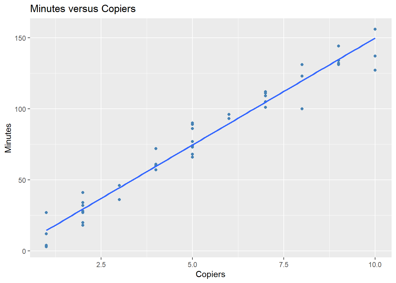
- Obtain a point estimate of the mean service time when 7 copiers are serviced.
predict(model, data.frame(Copiers = 7))
#>        1
#> 104.6666
- Obtain a 95% confidence interval for the slope.
confint(model, "Copiers", level = 0.95)
#>            2.5 %   97.5 %
#> Copiers 14.06101 16.00949
- Obtain a 95% confidence interval for the mean service time when 7 copiers are serviced.
predict(model, data.frame(Copiers = 7), interval = "confidence", level = 0.95)
#>        fit      lwr      upr
#> 1 104.6666 101.4159 107.9173
- Obtain a 95% prediction interval for the mean service time when 7 copiers are serviced.
predict(model, data.frame(Copiers = 7), interval = "prediction", level = 0.95)
#>        fit      lwr      upr
#> 1 104.6666 86.39922 122.9339