Introduction

R is a programming language and software environment for statistical analysis, graphics representation, and reporting. R was created by Ross Ihaka and Robert Gentleman at the University of Auckland, New Zealand, and is currently developed by the R Development Core Team. It is free of charge and open-source.

Nowadays, many companies, universities, and individuals of all backgrounds are shifting towards using R, because (of):

It is free and open-source, and available on every major platform.
Results produced by R are reproducible.
R has a diverse and supportive community, both online and offline.
A numerous set of packages for various tasks such as statistical analysis, data science, data visualization, reporting results etc.
Powerful tools for communicating your results.
RStudio IDE (Integrated Development Environment).
Deep-seated language support for data analysis.
A strong foundation of functional programming.

Getting Started: Downloading and Installing R & RStudio

Installing R

The first thing we need to do is to install R on your computer. It works on pretty much every platform available, including the widely used Windows, Mac OS, and Linux systems. You can download R here. Pick your operating system and follow the instructions stated on that page. After you download R, install it on your machine.

Installing RStudio

R itself has an old-fashion, old-school interface, which is less intuitive and makes coding harder (especially for beginners). Thus, we will be using RStudio instead. RStudio is an IDE (Integrated Development Environment), which has a user-friendly interface and is equipment with many useful features. It facilitates extensive code editing, development as well as various features that make R an easy language to implement. We will be using RStudio to call R. You can dowload RStudio here.

Note, in order to work in RStudio, you first need to download and install R.

RStudio Interface

You may be initially overwhelmed by all the different panes and tabs that are available in RStudio. But, as with all things, it will take a little bit to get used to it and eventually you will learn to love this layout.

RStudio has 4 main panes:

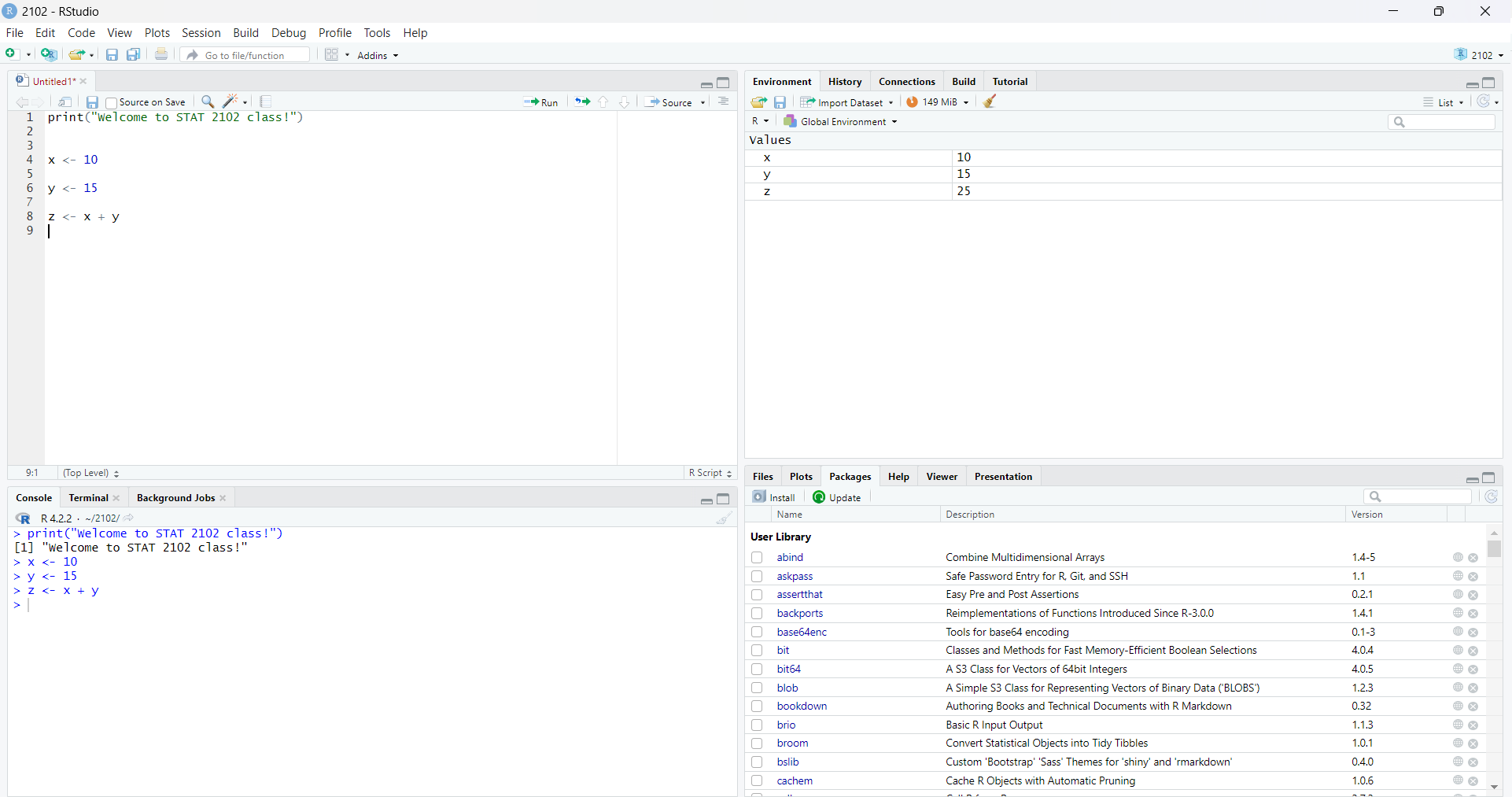
Code Editor (Source Pane)

Most likely the pane where you will spend a majority of your time is in the top left corner. It’s called Code Editor (a.k.a Source Pane). This is a place where you create and edit R Scripts (files with an ".R" extension that contain your code). When you open RStudio, it will automatically start a new Untitled script. Before you start typing in an untitled R script, you should always save the file under a new file name (for example, "script_1.R"). That way, if something on your computer crashes while you’re working, R will have your code saved when you re-open RStudio.

As you will notice, typing a code in R scripts does not execute it. To run the entire code, you can click a Run button on the top of the pane. Or, if you want to execute a specific line of the code, then put the cursor on that line and press Command + Return on Mac or Control + Enter on PC.

Console Pane

The bottom left pane is called Console. You will be using the Console as a way to check your work or thoughts. Basically, Console is a place where the R code is being run after executing it in R scripts. It is a place where the output/results will be displayed.

Environment/History Pane

The Environment (a.k.a Global Environment, a.k.a Working Environment) tab shows you the names of all the data objects that you’ve defined in your current R session. You can also see what information these objects contain.

The History tab simply shows you a history of all the code you’ve previously evaluated in the Console.

Output Pane

The bottom right pane in RStudio contains the most tabs by default and is a useful place to view a variety of miscellaneous information about your RStudio projects and its files.

Files: The leftmost tab here shows the file and folder structure. This shows you where the files are stored, what they are called, and any folders that may exist in your project folder.

Plots/Viewer: this shows you the resulting graphs/figures that your R code generated.

Packages: this shows you what packages have been downloaded to your computer. You can also see which packages are loaded into the current working environment by looking to see if a check-mark exists next to the package name.

Help: this shows you documentations on R functions, datasets, and packages available in R.

R as a Calculator: Operators

An operator is a symbol that tells R to perform specific mathematical or logical manipulations. R language is rich it built-in operators and provides the following types of operators:

Arithmetic Operators
Relational Operators
Logical Operators
Assignment Operators

In this module we consider arithmetic and assignment operators. Later on, we will discuss relational and logical ones.

Arithmetic Operators

R supports various arithmetic operations. In other words, you can use R as a simple calculator. For instance,

print(2 + 3)
#> [1] 5

print(4*5 - 2/3)
#> [1] 19.33333

The following table shows the basic arithmetic operators supported by R language:

R Symbol	Meaning	Example	Output
+	Addition	`5+3`	`8`
-	Subtraction	`5-3`	`2`
*	Multiplication	`5*3`	`15`
/	Division	`5/3`	`1.666667`
^	Exponents	`5^3`	`125`
%%	Remainder	`5%%3`	`2`
sqrt()	Square Root	`sqrt(5)`	`2.236068`
log( , base = )	Logarithm	`log(5, base = 3)`	`1.464974`
abs()	Absolute Value	`abs(-5)`	`5`

Assignment Operators

In order to create a variable in R, you can use <- assignment symbol. For example, let’s create a variable x and give it a value of 4:

x <- 4
print(x)
#> [1] 4

Let’s create another variable y, which is equal to 10:

y <- 10
print(y)
#> [1] 10

Once we create these variables, they will be stored in the global environment and will be available to use for further operations. Now R knows that x = 4 and y = 10.

print(x + y)
#> [1] 14

Note, R is case sensitive. What does that mean? This means that for R x and X are different objects. So, now if we call X variable, R will throw an error and will tell you that such an object does exist in the global environment:

print(X)
#> Error in eval(expr, envir, enclos): object 'X' not found

Working with a Global Environment

Saving the Global Environment

After you’ve run a long code and produced some valuable results, you might want to save your output that is being stored in the global environment now. To do so, you can execute the following line of code, which saves the global environment in the working directory (a place in your computer where R saves your files):

save.image()

Removing Objects from the Global Environment

To remove a specific object (suppose a variable x) from the Global Environment, use rm() function:

rm(x)

To remove all objects stored in the Global Environment, use rm(list = ls()) function:

rm(list = ls())

Listing Objects Stored in the Global Environment

To list the objects stored in the Global Environment, use ls() function:

ls()

Working Directory

As mentioned, R stores files in the working directory. To check where the working directory on your machine is, use getwd() function:

getwd()
#> [1] "C:/Users/alexp/OneDrive/Desktop/R Bootcamp/R_bootcamp"

Getting Help

Sometimes you don’t exactly know how certain functions work. You can use ? in the console followed by the function name to figure what the inputs (arguments) of this function are and how it can be utilized. For example, let’s check how the mean() function works:

?mean

Now in the output pane (bottom right pane) under Help tab you should see all information about the mean() function.

Welcome

Module 1