Lecture 17
Sampling Methods
When working on a research project/study, you always have a specific population of interest that you would like to target. For instance, if you want to do some research on everyone in North America, then all people living in North America will be the population of interest. Or, suppose you work for a manufacturing plant and you are interested in examining the quality of valves that this manufacturing plant produces. Then, all valves produced by this manufacturing plant will be your population of interest. In general, a population is the complete set of all objects or people of interest. In other words, it is a totality of the individuals of objects that are of interest in a statistical study.
Typically, you are interested in assessing certain characteristics of a population. These characteristics are summary values calculated from a population and are called population parameters. It is normally impractical to study a whole population to deterministically calculate population parameters, because we would need to observe every individual/object in the population and this procedure has some limitations (for instance, it might take too long to complete the study, the research costs are too high, or it might destroy all items in the population in the process of measurement).
Thus, instead of measuring/examining every element in a population, we take a sample. A sample is a subset of the elements that is often a small fraction of the overall population. For instance, instead of surveying all people in North America, we will take a sample of 10,000 people. Or, instead of examining all valves produced by the manufacturing plant, we will take a sample of 300 valves. Characteristics describing a sample are called sample statistics. We then use a sample statistic to estimate the corresponding population parameter.
In this lecture, we will discuss different sampling methods. As you already understand, sampling is a method that allows researchers to infer information about a population based on results from a subset of the population, without having to investigate every individual. Sampling is an essential part of any research project. The right sampling method can make or break the validity of your research, and it’s essential to choose the right method for your specific question.
If a sample is to be used, by whatever method it is chosen, it is important that the individuals/objects selected are representative of the whole population. The best way to ensure a sample is representative of the population is to ensure all the observations that comprise it were selected at random. Representative samples allow us to generalize the results from the sample to the population.
There are several different sampling techniques available, and they can be subdivided into two groups: probability sampling and non-probability sampling. In probability (random) sampling, you start with a complete sampling frame of all eligible individuals from which you select your sample. In this way, all eligible individuals have a chance of being chosen for the sample, and you will be more able to generalise the results from your study. Probability sampling methods tend to be more time-consuming and expensive than non-probability sampling.
In non-probability (non-random) sampling, you do not start with a complete sampling frame, so some individuals have no chance of being selected. Consequently, you cannot estimate the effect of sampling error and there is a significant risk of ending up with a non-representative sample which produces non-generalisable results. However, non-probability sampling methods tend to be cheaper and more convenient, and they are useful for exploratory research and hypothesis generation.
Probability Sampling Methods
Consider the salaries of Major League Baseball (MLB) players, where each player is a member of one of 30 teams. We would like to know what an average salary of MLB player is. In this example, all MLB players are a population of interest and their average salary is a population parameter. Now you know that you have to take a sample from the population of all MLB players in order to estimate their average salary. But how can we do that?
Below we discuss different sampling methods that you can utilize.
Simple Random Sampling
A Simple Random Sample (SRS) from a population is one in which each possible sample of that size has the same chance of selection. In other words, every member of the population has the exact same chance of being selected into the sample. In this case each individual is chosen entirely by chance. SRS is a good way of ensuring that your sample is representative of the population it is chosen from.
One way of obtaining a random sample is to give each individual in a population a number, and then use a table of random numbers to decide which individuals to include. Or, for instance, in our example we might write last year’s salary for each of the MLB players on a scrap of paper and randomly jumble them in a bag. Thereafter, we could blindly pull a sample of these paper scraps out of the bag.
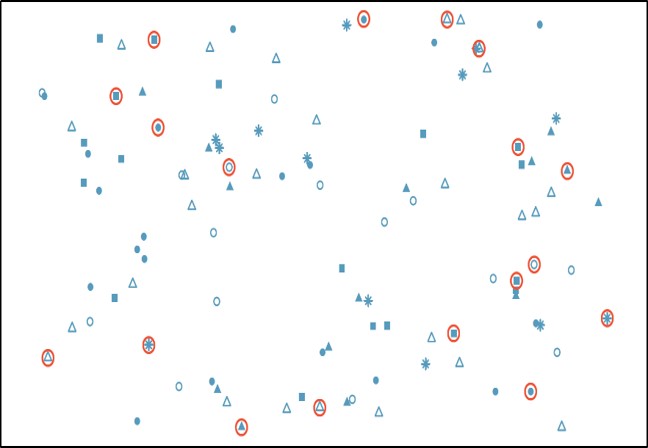
A specific advantage of SRS is that it is the most straightforward method of probability sampling. A disadvantage of simple random sampling is that you may not select enough individuals with your characteristic of interest, especially if that characteristic is uncommon.
Stratified Sampling
In this method, the population is first divided into subgroups (or strata) who all share a similar characteristic. Thereafter, a simple random sample (SRS) is taken from each stratum. It is used when we might reasonably expect the measurement of interest to vary between the different subgroups, and we want to ensure representation from all the subgroups. This method works best when there is a lot of variability between each stratum, but not much variability within each one.
In our example, instead of randomly sampling from the population of MLB salaries blindly, we could categorize (stratify) the salaries according to the position played by each player (pitcher, short-stop, catcher, etc.) Ideally, all the observations in each stratum are similar with respect to the outcome of interest.
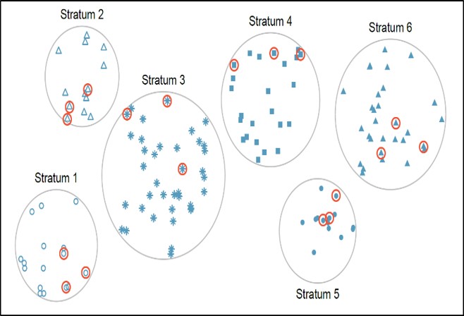
Stratified sampling improves the accuracy and representativeness of the results by reducing sampling bias. However, it requires knowledge of the appropriate characteristics of the sampling frame (the details of which are not always available), and it can be difficult to decide which characteristic(s) to stratify by.
Clustered Sampling
In a clustered sample, subgroups of the population are used as the sampling unit, rather than individuals. The population is divided into subgroups, known as clusters, which are randomly selected to be included in the study. This method works best when there is a lot of variability within each cluster and not a lot of variability between each cluster.
In our example, we could cluster players by their teams, then randomly select a few of these clusters (teams) and then observe all the players in the chosen clusters.
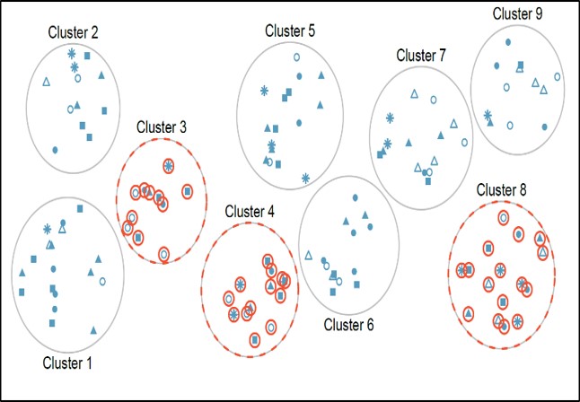
Cluster sampling can be more efficient than simple random sampling, especially where a study takes place over a wide geographical region. Disadvantages include an increased risk of bias, if the chosen clusters are not representative of the population, resulting in an increased sampling error.
Systematic Sampling
In systematic sampling, individuals are selected at regular intervals from the sampling frame. The intervals are chosen to ensure an adequate sample size. Specifically, we randomly select a fixed starting point and then select every k-th observation in the ordered population to be in the sample (where k is the population size divided by the desired sample size). Systematic sampling works well when your population can be ordered in some way. It is similar to SRS, since every member of the population has an equal chance of being chosen. But it is not the same as SRS, since not every possible sample has the same probability of being selected.
In our example, we can first order all MLB players by their last names. Then we would choose a random number between 1 and 15 as a starting point, and then select every 15-th person on the list to be in our sample.
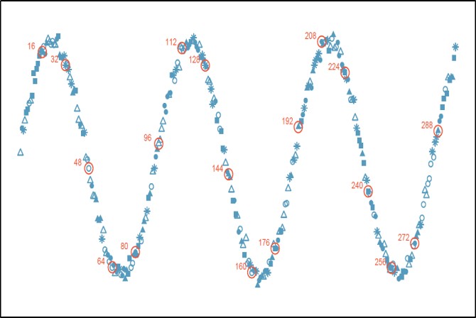
Systematic sampling is often more convenient than simple random sampling, and it is easy to administer. However, it may also lead to bias, for example if there are underlying patterns in the order of the individuals in the sampling frame, such that the sampling technique coincides with the periodicity of the underlying pattern.
Non-Probability Sampling Methods
Convenience Sampling
Convenience sampling is perhaps the easiest method of sampling, because participants are selected based on availability and willingness to take part. Useful results can be obtained, but the results are prone to significant bias, because those who volunteer to take part may be different from those who choose not to (volunteer bias), and the sample may not be representative of other characteristics, such as age or sex.
Note: volunteer bias is a risk of all non-probability sampling methods. Thus, while it’s possible to get interesting information from a convenience sample, they are rarely (if ever) representative of a larger population.
In our example, we could browse websites and collect salaries of several MLB players that are publicly available.
Practice Problems: Guess the Sampling Method
A third-grade teacher has a bag of craft sticks. Each stick has the name of one student in the class written on it. To select three students to help with a school assembly the teacher reaches into the bag without looking and chooses 3 sticks.
A researcher studying short-term memory believes that age plays a role. From a large group of people who have agreed to be part of a research study, the researcher randomly selects 40 people over the age of 50, 40 people between the ages of 30 and 50, and 40 people who are between the ages of 15 and 30.
Marcus and Caroline are collecting data about the price of soda and candy bars at service stations. They collect the information from the service stations that are close enough to their house to ride their bikes to.
Columbia University housing officials want to collect in-depth information about student life on campus. They create a list of every floor of every dorm on campus, and then randomly select 4 floors from the list and survey every resident on those 4 floors.
To select a sample of 12 Kentucky Derby winning horses, we arrange the winner by year, select a random number between 1 and 10, and then include that horse and every 10th horse on the list.
Motivated by a student who died from binge drinking, the administration at a university conducts a study of student drinking by randomly selecting 10 different classes being taught this semester and interviewing all of the students in each of those classes.
Answers:
Simple Random Sampling
Stratified Sampling
Convenience Sampling
Clustered Sampling
Systematic Sampling
Clustered Sampling
Sampling with R
For illustrative purposes, we will be using Diamonds and Attritiondatasets. Below are brief descriptions of these datasets:
Diamonds - a dataset (available in ggplot2 package) containing the prices and other attributes of almost 54,000 diamonds with the following variables:
-
carat- Weight of the diamond -
cut- Quality of the cut (a categorical variable with Fair, Good, Very Good, Premium, Ideal levels) -
color- Diamond color (a categorical variable with levels from D (best) to J (worst)) -
clarity- A measurement of how clear the diamond is (a categorical variable with I1 (worst), SI2, SI1, VS2, VS1, VVS2, VVS1, IF (best) levels) -
table- Width of top of diamond relative to widest point -
price- Price in US dollars -
length- Length in mm -
width- Width in mm -
depth- Depth in mm
head(diamonds)
#> # A tibble: 6 × 10
#>   carat cut      color clarity depth table price     x     y
#>   <dbl> <ord>    <ord> <ord>   <dbl> <dbl> <int> <dbl> <dbl>
#> 1  0.23 Ideal    E     SI2      61.5    55   326  3.95  3.98
#> 2  0.21 Premium  E     SI1      59.8    61   326  3.89  3.84
#> 3  0.23 Good     E     VS1      56.9    65   327  4.05  4.07
#> 4  0.29 Premium  I     VS2      62.4    58   334  4.2   4.23
#> 5  0.31 Good     J     SI2      63.3    58   335  4.34  4.35
#> 6  0.24 Very Go… J     VVS2     62.8    57   336  3.94  3.96
#> # ℹ 1 more variable: z <dbl>
Attrition - a dataset (available in tidymodels package) containing employee attrition information originally provided by IBM Watson Analytics Lab. It contains 1470 observations and 31 variables, among which:
-
Attrition- Employee attrition (a categorical variable with Yes and No levels) -
Age- Employee’s age -
Gender- Employee’s gender -
MonthlyIncome- Employee’s monthly income -
OverTime- A categorical variable indicating whether an employee worked overtime (Yes/No) and more ...
library(tidymodels)
#> Warning: package 'tidymodels' was built under R version
#> 4.4.3
#> ── Attaching packages ────────────────── tidymodels 1.3.0 ──
#> ✔ broom        1.0.7     ✔ rsample      1.3.0
#> ✔ dials        1.4.0     ✔ tune         1.3.0
#> ✔ infer        1.0.7     ✔ workflows    1.2.0
#> ✔ modeldata    1.4.0     ✔ workflowsets 1.1.0
#> ✔ parsnip      1.3.1     ✔ yardstick    1.3.2
#> ✔ recipes      1.2.1
#> Warning: package 'dials' was built under R version 4.4.3
#> Warning: package 'infer' was built under R version 4.4.3
#> Warning: package 'modeldata' was built under R version
#> 4.4.3
#> Warning: package 'parsnip' was built under R version 4.4.3
#> Warning: package 'recipes' was built under R version 4.4.3
#> Warning: package 'rsample' was built under R version 4.4.3
#> Warning: package 'tune' was built under R version 4.4.3
#> Warning: package 'workflows' was built under R version
#> 4.4.3
#> Warning: package 'workflowsets' was built under R version
#> 4.4.3
#> Warning: package 'yardstick' was built under R version
#> 4.4.3
#> ── Conflicts ───────────────────── tidymodels_conflicts() ──
#> ✖ scales::discard() masks purrr::discard()
#> ✖ dplyr::filter()   masks stats::filter()
#> ✖ recipes::fixed()  masks stringr::fixed()
#> ✖ dplyr::lag()      masks stats::lag()
#> ✖ yardstick::spec() masks readr::spec()
#> ✖ recipes::step()   masks stats::step()

attrition <- attrition

head(attrition)
#>   Age Attrition    BusinessTravel DailyRate
#> 1  41       Yes     Travel_Rarely      1102
#> 2  49        No Travel_Frequently       279
#> 4  37       Yes     Travel_Rarely      1373
#> 5  33        No Travel_Frequently      1392
#> 7  27        No     Travel_Rarely       591
#> 8  32        No Travel_Frequently      1005
#>             Department DistanceFromHome     Education
#> 1                Sales                1       College
#> 2 Research_Development                8 Below_College
#> 4 Research_Development                2       College
#> 5 Research_Development                3        Master
#> 7 Research_Development                2 Below_College
#> 8 Research_Development                2       College
#>   EducationField EnvironmentSatisfaction Gender HourlyRate
#> 1  Life_Sciences                  Medium Female         94
#> 2  Life_Sciences                    High   Male         61
#> 4          Other               Very_High   Male         92
#> 5  Life_Sciences               Very_High Female         56
#> 7        Medical                     Low   Male         40
#> 8  Life_Sciences               Very_High   Male         79
#>   JobInvolvement JobLevel               JobRole
#> 1           High        2       Sales_Executive
#> 2         Medium        2    Research_Scientist
#> 4         Medium        1 Laboratory_Technician
#> 5           High        1    Research_Scientist
#> 7           High        1 Laboratory_Technician
#> 8           High        1 Laboratory_Technician
#>   JobSatisfaction MaritalStatus MonthlyIncome MonthlyRate
#> 1       Very_High        Single          5993       19479
#> 2          Medium       Married          5130       24907
#> 4            High        Single          2090        2396
#> 5            High       Married          2909       23159
#> 7          Medium       Married          3468       16632
#> 8       Very_High        Single          3068       11864
#>   NumCompaniesWorked OverTime PercentSalaryHike
#> 1                  8      Yes                11
#> 2                  1       No                23
#> 4                  6      Yes                15
#> 5                  1      Yes                11
#> 7                  9       No                12
#> 8                  0       No                13
#>   PerformanceRating RelationshipSatisfaction
#> 1         Excellent                      Low
#> 2       Outstanding                Very_High
#> 4         Excellent                   Medium
#> 5         Excellent                     High
#> 7         Excellent                Very_High
#> 8         Excellent                     High
#>   StockOptionLevel TotalWorkingYears TrainingTimesLastYear
#> 1                0                 8                     0
#> 2                1                10                     3
#> 4                0                 7                     3
#> 5                0                 8                     3
#> 7                1                 6                     3
#> 8                0                 8                     2
#>   WorkLifeBalance YearsAtCompany YearsInCurrentRole
#> 1             Bad              6                  4
#> 2          Better             10                  7
#> 4          Better              0                  0
#> 5          Better              8                  7
#> 7          Better              2                  2
#> 8            Good              7                  7
#>   YearsSinceLastPromotion YearsWithCurrManager
#> 1                       0                    5
#> 2                       1                    7
#> 4                       0                    0
#> 5                       3                    0
#> 7                       2                    2
#> 8                       3                    6
Simple Random Sampling
As it was mentioned, the simplest way of doing sampling is to take a simple random sample. This does not control for any data attributes, such as the distribution of your response variable Y. For instance, let’s consider the Diamonds dataset. The target (response) variable in the dataset is price, a price of diamonds given in US dollars.
Typically, as discussed earlier, if a sample is to be used, by whatever method it is chosen, it is important that the individuals/objects selected are representative of the whole population. Normally, you would want your sample to preserve the distribution of the target variable. In other words, the distribution of the target variable in a sample should be somewhat similar to the population distribution of the target variable.
Most of the time, a simple random sample does a good job in preserving the target distribution (for sufficiently large sample size). To take a simple random sample, we will use initial_split() and training() functions from the rsample package (rsample package is a part of tidymodels package, thus, to activate rsample it is enough to install the tidymodels package and load it into R).
initial_split creates a single binary split of the data into a training set and testing set (later you will see what these training and testing datasets mean) and training is used to extract the resulting data.
For example, let’s take a simple random sample from the Diamonds datasets containing 20% of the original data.
library(tidymodels)

set.seed(1)

sample_SRS <- diamonds %>% initial_split(prop = 0.2) %>% training()
To see how well the target distribution was preserved in the sample, we can plot a histogram of the target distribution for both original and sample data side-by-side:
library(patchwork)
#> Warning: package 'patchwork' was built under R version
#> 4.4.3


original <- ggplot(data = diamonds) +

            geom_histogram(aes(x = price),

                           fill = "tomato") +

            labs(title = "Histogram of Price (original data)",

                 x = "Price",

                 y = "Frequency")


sample <- ggplot(data = sample_SRS) +

            geom_histogram(aes(x = price),

                           fill = "tomato") +

            labs(title = "Histogram of Price (sample data)",

                 subtitle =  "Simple Random Sampling (SRS)",

                 x = "Price",

                 y = "Frequency")


original + sample
#> `stat_bin()` using `bins = 30`. Pick better value with
#> `binwidth`.
#> `stat_bin()` using `bins = 30`. Pick better value with
#> `binwidth`.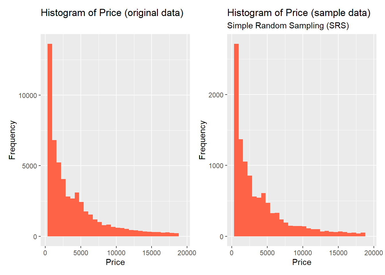
You can see that the original and sample distributions of the target variable are almost identical. Thus, for this case, SRS does a great job in preserving the underlying distribution.
Systematic Sampling
To take a systematic sample from our data, we have to first order the dataset in some way, select a fixed starting point, and then select every k-th observation in the ordered population.
Let’s use the price variable to re-order the observations in the dataset in descending order. Then, we will select every 5-th observation in the dataset starting from the 1-st observation (in this case k = 5, because we want our sample to contain 20% of original data):
library(patchwork)


original <- ggplot(data = diamonds) +

            geom_histogram(aes(x = price),

                           fill = "tomato") +

            labs(title = "Histogram of Price (original data)",

                 x = "Price",

                 y = "Frequency")


sample <- ggplot(data = sample_sys) +

            geom_histogram(aes(x = price),

                           fill = "tomato") +

            labs(title = "Histogram of Price (sample data)",

                 subtitle =  "Systematic Sampling",

                 x = "Price",

                 y = "Frequency")


original + sample
#> `stat_bin()` using `bins = 30`. Pick better value with
#> `binwidth`.
#> `stat_bin()` using `bins = 30`. Pick better value with
#> `binwidth`.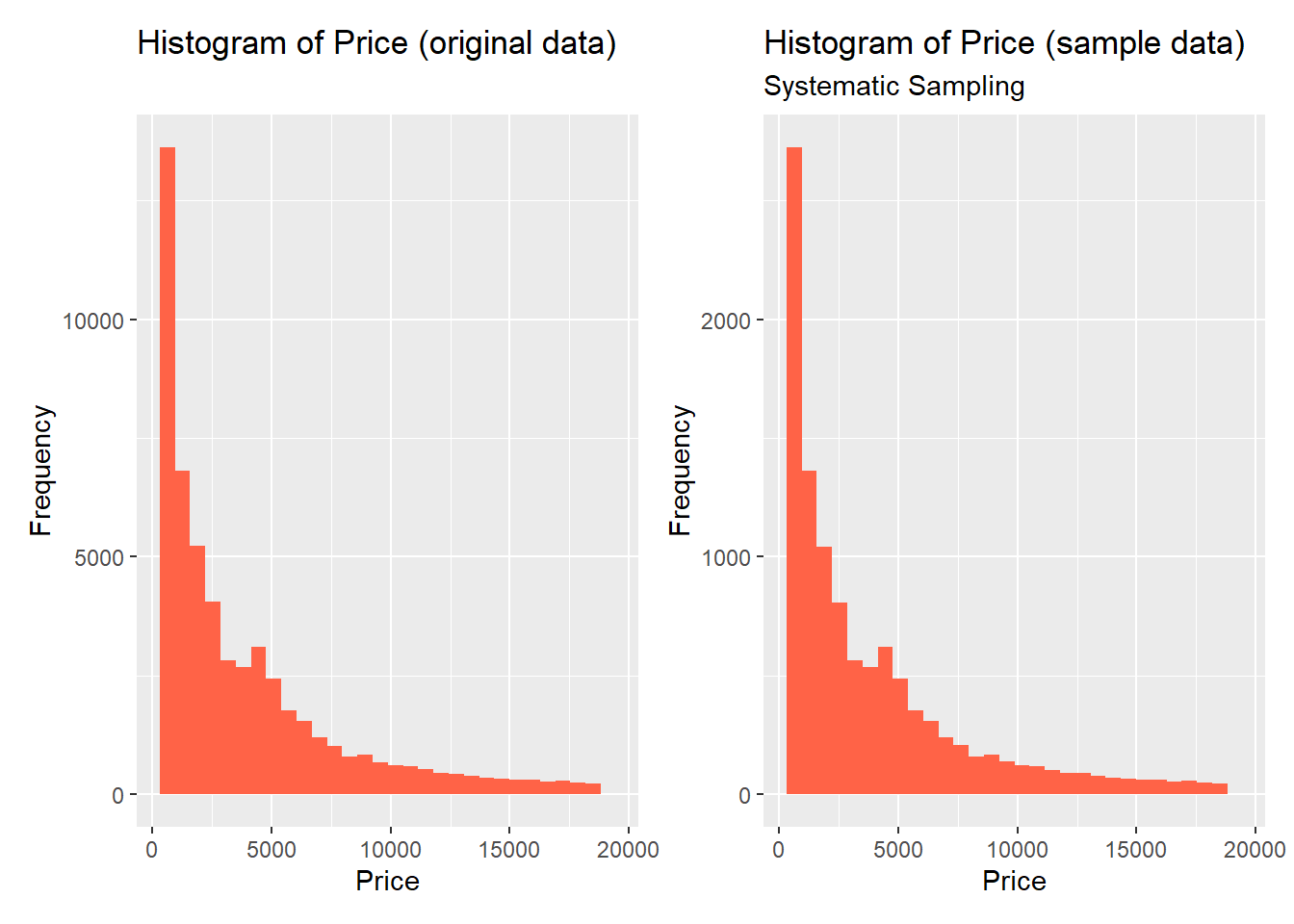
Once again, we can observe that the original and sample distributions of the target variable are almost identical.
Stratified Sampling
Sometimes a target variable in your data is a categorical variable (a factor). This is more common with classification problems, where you aim to predict a class of a new observation. A categorical variable can be severely imbalanced (vast majority of observations belong to one category of the variable, and the remaining observations are spread across the other levels).
Attrition dataset is one of such examples. Here, roughly 84% of the observations belong to No category and the remaining 16% of observations belong to Yes category.
In this scenario, we would want to explicitly control the underlying distribution of the target variable in our sample. Thus, simple random sampling might not be the best choice since it fails to do so. For instance, if we randomly select 20% of the observations (like SRS does), we might end up having all observations taken from one single category, and, as a result, our sample will no longer be representative.
In such cases, the solutions is using stratified sampling. To take a stratified sample, you need to add strata argument to the initial_split function and pass the name of variable whose distribution you want to preserve in a sample:
set.seed(1)

sample_strata <- attrition %>%

                 initial_split(prop = 0.2, strata = Attrition) %>%

                 training()
library(patchwork)


original <- ggplot(data = attrition) +

geom_bar(mapping = aes(x = Attrition),

         fill = "orange",

         width = 0.9) +

geom_text(aes(x = Attrition,label = scales::percent((..count..)/sum(..count..))),

            stat = "count",

            vjust = 1.5,

            size = 6,

            colour = "white") +

  labs(title = "Original Dataset")


sample <- ggplot(data = sample_strata) +

geom_bar(mapping = aes(x = Attrition),

         fill = "orange",

         width = 0.9) +

geom_text(aes(x = Attrition,label = scales::percent((..count..)/sum(..count..))),

            stat = "count",

            vjust = 1.5,

            size = 6,

            colour = "white")+

  labs(title = "Stratified Sample")


original + sample
#> Warning: The dot-dot notation (`..count..`) was deprecated in
#> ggplot2 3.4.0.
#> ℹ Please use `after_stat(count)` instead.
#> This warning is displayed once every 8 hours.
#> Call `lifecycle::last_lifecycle_warnings()` to see where
#> this warning was generated.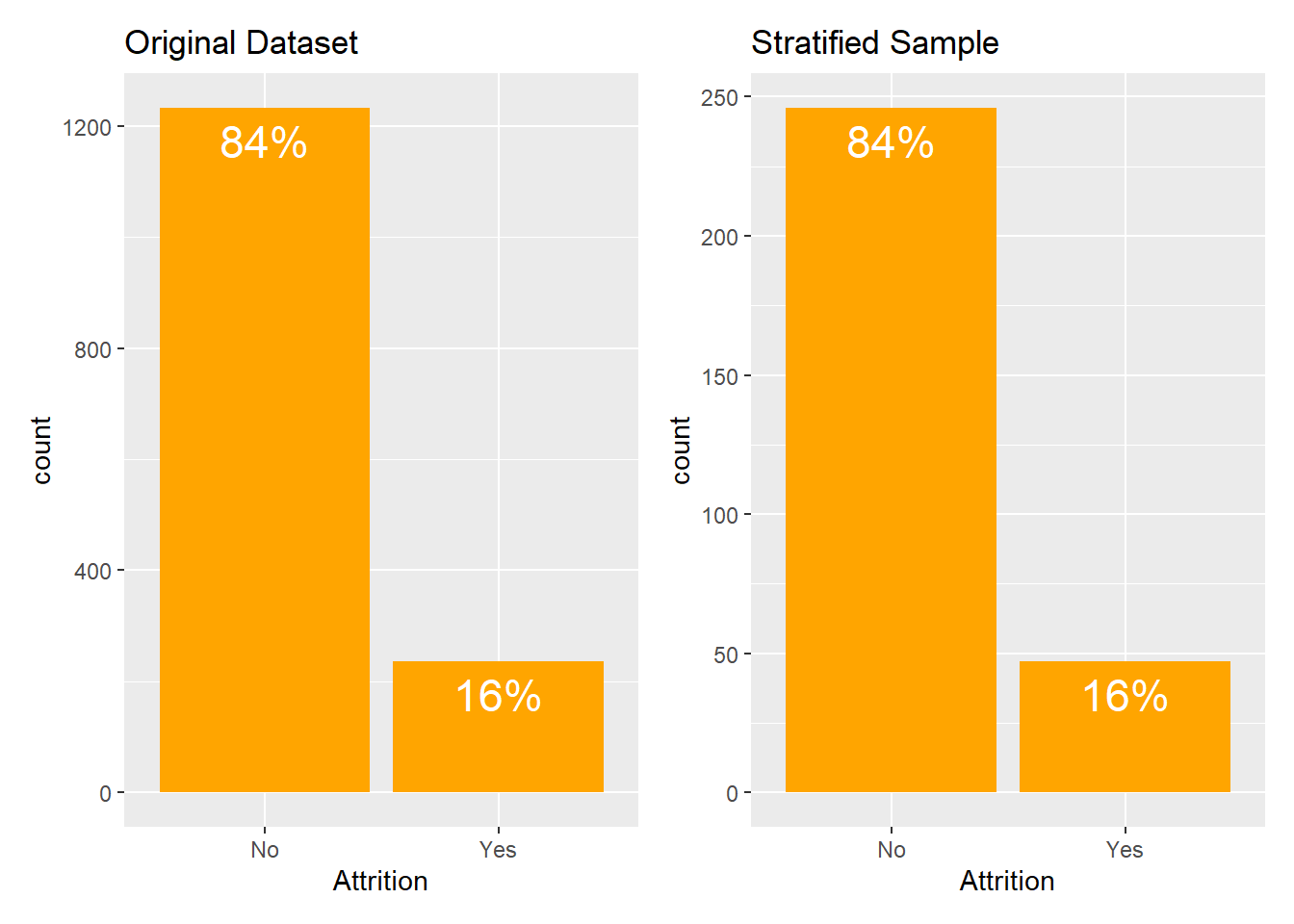
As illustrated in the barplots above, stratified sampling method perfectly preserves the underlying distribution of the Attrition variable.
Resampling Methods
There are several steps to creating a useful model, including parameter estimation, model selection and tuning, and performance assessment. At the start of a new project, there is usually an initial finite pool of data available for all these tasks, which we can think of as an available data budget. How should the data be applied to different steps or tasks? The idea of data spending is an important first consideration when modeling, especially as it relates to empirical validation.
Approaching model-building process correctly means approaching it strategically by spending our data wisely on learning and validation procedures, properly pre-processing the feature and target variables, minimizing data leakage, tuning hyperparameters, and assessing model performance.
In this section we will discuss basics of data splitting.
Data Splitting
A major goal of any model-building process is to find an algorithm that most accurately predicts future values of the response variable Y based on a set of predictor variables Xs. In other words, we want an algorithm that not only fits well to our past data, but more importantly, one that predicts a future outcome accurately. This is called the generalizability of our algorithm. How we “spend” our data will help us understand how well our algorithm generalizes to unseen data.
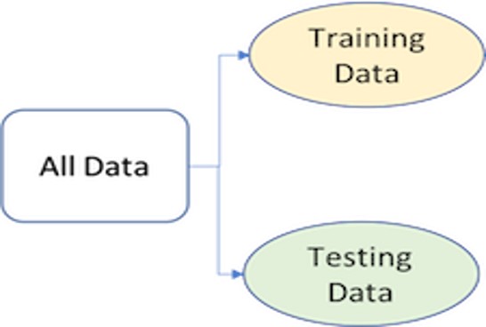
To provide an accurate understanding of the generalizability of our final optimal model, we can split our data into training and test data sets:
Training set: this data is used to develop feature sets, train our algorithms, tune hyperparameters, compare models, and all of the other activities required to choose a final model (e.g., the model we want to put into production).
Test set: having chosen a final model, this data is used to estimate an unbiased assessment of the model’s performance, which we refer to as the generalization error.
Note: it is critical that the test set not be used prior to selecting your final model. Assessing results on the test set prior to final model selection biases the model selection process since the testing data will have become part of the model development process.
Given a fixed amount of data, typical recommendations for splitting your data into training-test splits include 60% (training)–40% (testing), 70%–30%, or 80%–20%. Generally speaking, these are appropriate guidelines to follow; however, it is good to keep the following points in mind:
Spending too much in training (e.g., >80%) won’t allow us to get a good assessment of predictive performance. We may find a model that fits the training data very well, but is not generalizable (overfitting).
Sometimes too much spent in testing ( >40%) won’t allow us to get a good assessment of model parameters (underfitting).
The two most common ways of splitting data include Simple Random Sampling and Stratified Sampling.
Sometimes imbalanced data can have a significant impact on model predictions and performance. Most often this involves classification problems where one class has a very small proportion of observations (e.g., defaults - 5% versus nondefaults - 95%). Several sampling methods have been developed to help remedy class imbalance and most of them can be categorized as either up-sampling or down-sampling.
Down-sampling balances the dataset by reducing the size of the abundant class(es) to match the frequencies in the least prevalent class. This method is used when the quantity of data is sufficient. By keeping all samples in the rare class and randomly selecting an equal number of samples in the abundant class, a balanced new dataset can be retrieved for further modeling. Furthermore, the reduced sample size reduces the computation burden imposed by further steps in the model-building process.
On the contrary, up-sampling is used when the quantity of data is insufficient. It tries to balance the dataset by increasing the size of rarer samples. Rather than getting rid of abundant samples, new rare samples are generated by using repetition or bootstrapping (discussed later). Note that there is no absolute advantage of one sampling method over another. Application of these two methods depends on the use case it applies to and the data set itself.
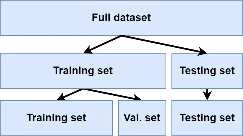
So far we’ve discussed splitting our data into training and testing sets. Furthermore, we were very explicit about the fact that we do not use the test set to assess model performance during the training phase. So how do we assess the generalization performance of the model?
Solution 1: Assess the model performance based on the training data. Disadvantages - this leads to biased results as some models can perform very well on the training data but not generalize well to a new data set (overfitting).
Solution 2: Use a validation approach, which involves splitting the training set further to create two parts: a training set and a validation set (a.k.a. holdout set). Disadvantages - validation using a single holdout set can be highly variable and unreliable unless you are working with very large data sets.
Solution 3: Resampling methods. They allow to repeatedly fit a model to parts of the training data and test its performance on other parts. The two commonly used resampling methods include k-fold cross validation and bootstrapping.
k-fold cross validation
k-fold cross-validation (aka k-fold CV) is a resampling method that randomly divides the training data into k groups (aka folds) of approximately equal size. The model is fit on k-1 folds and then the remaining fold is used to compute model performance.
This procedure is repeated k times; each time, a different fold is treated as the validation set. This process results in k estimates of the generalization error. Thus, the k-fold CV estimate is computed by averaging the k test errors, providing us with an approximation of the error we might expect on unseen data.
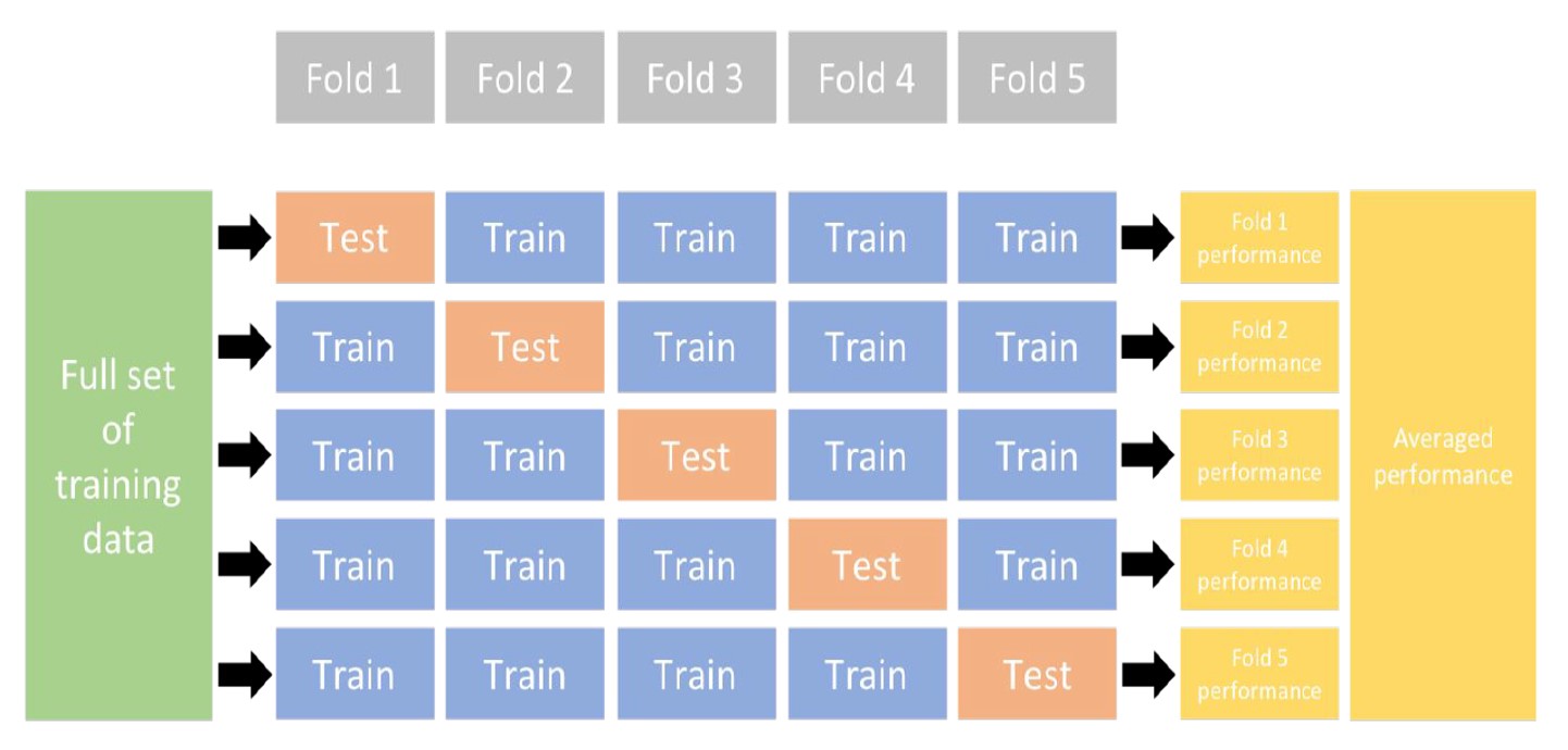
Consequently, with k-fold CV, every observation in the training data will be held out one time to be included in the test set as illustrated in the figure above. In practice, one typically uses k = 5 or k = 10. There is no formal rule as to the size of k; however, as k gets larger, the difference between the estimated performance and the true performance to be seen on the test set will decrease. On the other hand, using too large k can introduce computational burdens.
One special variation of cross-validation is Leave-One-Out (LOO) Cross-Validation. If there are n training set samples, n models (n folds) are fit using n − 1 observations from the training set. Each model predicts the single excluded data point. At the end of resampling, the n predictions are pooled to produce a single performance statistic.
Leave-one-out methods are deficient compared to almost any other method. For anything but pathologically small samples, LOO is computationally excessive, and it may not have good statistical properties.
Bootstrapping
A bootstrap sample is a random sample of the data taken with replacement. This means that, after a data point is selected for inclusion in the subset, it’s still available for further selection. A bootstrap sample is the same size as the original data set from which it was constructed.
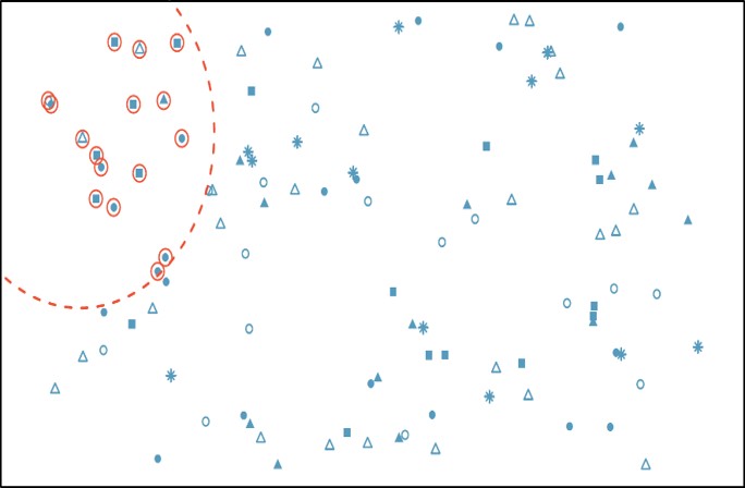
The figure below provides a schematic of bootstrap sampling where each bootstrap sample contains 12 observations just as in the original data set. Furthermore, bootstrap sampling will contain approximately the same distribution of values (represented by colors) as the original data set.
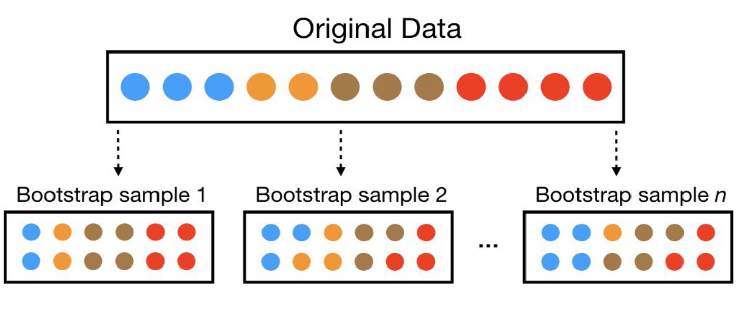
Since samples are drawn with replacement, each bootstrap sample is likely to contain duplicate values. In fact, on average, approximately 63.21% of the original sample ends up in any particular bootstrap sample. The original observations not contained in a particular bootstrap sample are considered out-of-bag (OOB). When bootstrapping, a model can be built on the selected samples and validated on the OOB samples.
Model Evaluation
Today, it has become widely accepted that a more sound approach to assessing model performance is to assess the predictive accuracy via loss functions. Loss functions are metrics that compare the predicted values to the actual value. When performing resampling methods, we assess the predicted values for a validation set compared to the actual target value.
For example, in regression, one way to measure error is to take the difference between the actual and predicted value for a given observation (this is the usual definition of a residual in ordinary linear regression). The overall validation error of the model is computed by aggregating the errors across the entire validation data set.
There are many loss functions to choose from when assessing the performance of a predictive model, each providing a unique understanding of the predictive accuracy and differing between regression and classification models. Furthermore, the way a loss function is computed will tend to emphasize certain types of errors over others and can lead to drastic differences in how we interpret the “optimal model”.
Its important to consider the problem context when identifying the preferred performance metric to use. And when comparing multiple models, we need to compare them across the same metric.
Depending on the problem context, we can divide them into two groups: Regression and Classification problems.
Regression Metrics
MSE - Mean Squared Error: Mean squared error is the average of the squared error (\(MSE = \frac{\sum_{i=1}^{n}(y_i - \hat{y_i})^2}{n}\)). The squared component results in larger errors having larger penalties. This (along with RMSE) is the most common error metric to use. Objective: minimize
RMSE - Root Mean Squared Error: Root mean squared error. This simply takes the square root of the MSE metric (\(RMSE =\sqrt{ \frac{\sum_{i=1}^{n}(y_i - \hat{y_i})^2}{n}}\)) so that your error is in the same units as your response variable. If your response variable units are dollars, the units of MSE are dollars-squared, but the RMSE will be in dollars. Objective: minimize
\(R^2\): This is a popular metric that represents the proportion of the variance in the dependent variable that is predictable from the independent variable(s). Unfortunately, it has several limitations. For example, two models built from two different data sets could have the exact same RMSE but if one has less variability in the response variable then it would have a lower \(R^2\) than the other. You should not place too much emphasis on this metric. Objective: maximize
Classification Metrics
Before we discuss evaluation metrics for classification problems, I would like to introduce a confusion matrix. In the field of statistics and machine learning, a confusion matrix is a table that visualizes the performance of a model. Each row of the confusion matrix represents the instances in an actual class while each column represents the instances in a predicted class, or vice versa (both variants are accepted and found in the literature).
It is a special kind of contingency table, with two dimensions (“actual” and “predicted”), and identical sets of “classes” in both dimensions (each combination of dimension and class is a variable in the contingency table):
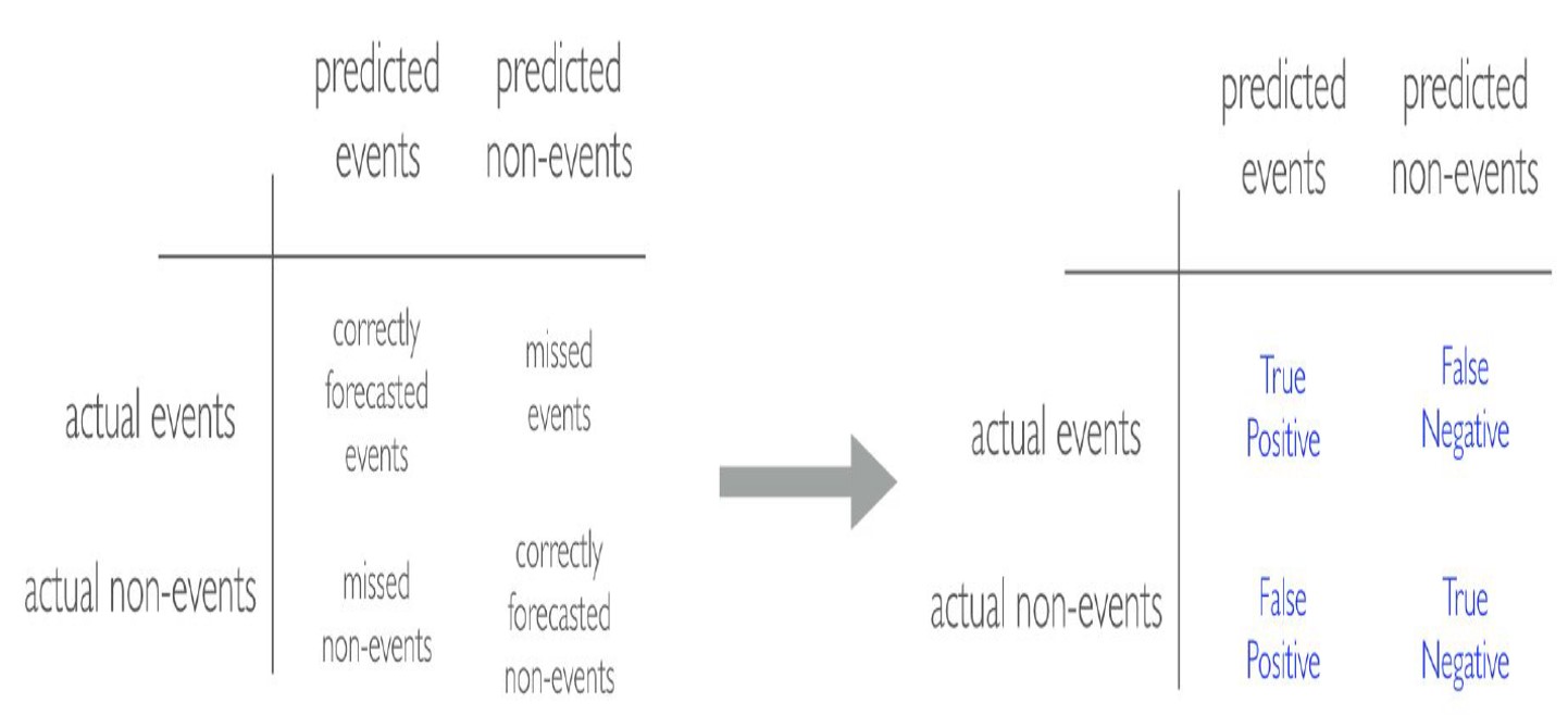
- Accuracy: accuracy tells you, overall, how often the classifier is correct.
\[\begin{align*} Accuracy = \frac{TP + TN}{Total} \end{align*}\]
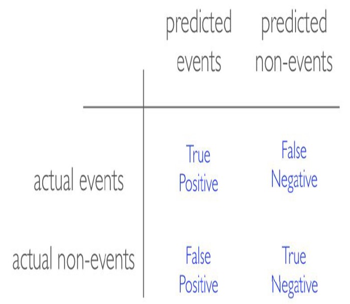
- Sensitivity (aka Recall): sensitivity tells you how accurately the classifier classifies actual events.
\[\begin{align*} Sensitivity = \frac{TP}{TP + FN} \end{align*}\]
- Specificity: specificity tells you how accurately the classifier classifies actual non-events.
\[\begin{align*} Specificity = \frac{TN}{FP + TN} \end{align*}\]
- Precision: precision tells you how accurately the classifier predicts actual events.
\[\begin{align*} Precision = \frac{TP}{TP + FP} \end{align*}\]